
GitHub Repository | PyPI Package
Machine learning often relies on complex models that act as black boxes, which makes interpretation difficult. Eigen-Component Analysis (ECA) takes inspiration from quantum theory to build interpretable linear models for classification and clustering. This article introduces the core idea, shows basic usage, and outlines the main parameters exposed by the eigen-analysis package.
Table of Contents
What is Eigen-Component Analysis?
Eigen-Component Analysis applies ideas inspired by quantum theory to create linear models for classification and clustering. Unlike many traditional preprocessing-heavy methods, ECA is designed to work without requiring data centralization or standardization, which can make the workflow simpler and the learned representation easier to inspect.
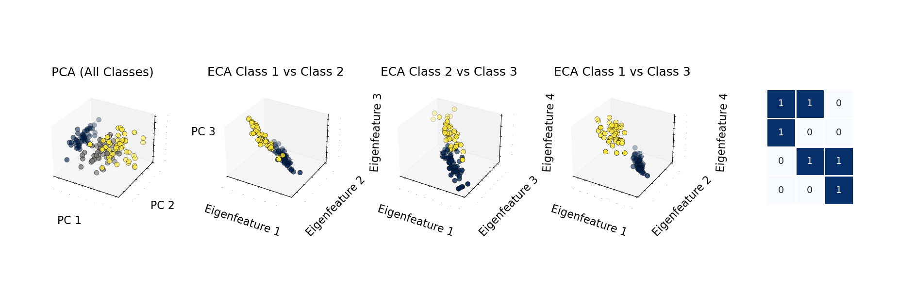
The central appeal of ECA is interpretability. The model exposes feature-to-class mappings through eigencomponents, giving researchers and data scientists a way to inspect why a prediction or cluster assignment is being made.
Key Features and Advantages
ECA combines theoretical structure with a practical Python implementation:
- Scikit-learn compatible interface: The package implements the familiar scikit-learn Estimator API, making it accessible to users already working in Python’s machine learning ecosystem.
- Supervised and unsupervised modes: ECA supports supervised classification and unsupervised clustering through related implementations:
ECAandUECA. - PyTorch backend: The implementation is built on PyTorch and can use GPU acceleration when a compatible CUDA device is available.
- Visualization tools: The package includes plotting utilities for eigenfeatures, feature mappings, training curves, and clustering or classification results.
- Mathematical foundation: ECA uses antisymmetric transformation matrices to build model representations inspired by quantum-theoretic structure.
Getting Started with ECA
Install the package from PyPI, or install it from source if you want to inspect or modify the implementation:
# Installation from PyPI
pip install eigen-analysis

# Or from source
git clone https://github.com/lachlanchen/eca.git
cd eca
pip install .
The package depends on common data science libraries, including NumPy, PyTorch, Matplotlib, Seaborn, scikit-learn, and SciPy. To verify the local installation, check that Python can import the package:
python - <<'PY'
import eigen_analysis
print("eigen_analysis imported successfully")
PY
Using ECA for Classification
The following example trains an ECA classifier on the classic Iris dataset:
# iris_classification.py
import traceback

import numpy as np
from eigen_analysis import ECA
from eigen_analysis.visualization import visualize_clustering_results
from sklearn import datasets
from sklearn.metrics import accuracy_score
from sklearn.model_selection import train_test_split

# Set random seed for reproducibility.
np.random.seed(23)

try:
    # Load Iris dataset.
    iris = datasets.load_iris()
    X = iris.data
    y = iris.target

    # Split data.
    X_train, X_test, y_train, y_test = train_test_split(
        X,
        y,
        test_size=0.2,
        random_state=23,
        stratify=y,
    )

    # Create and train ECA model.
    eca = ECA(num_clusters=3, num_epochs=10000, learning_rate=0.001)
    eca.fit(X_train, y_train)

    # Make predictions.
    y_pred = eca.predict(X_test)

    # Evaluate accuracy.
    accuracy = accuracy_score(y_test, y_pred)
    print(f"Test accuracy: {accuracy:.4f}")

    # Get transformed data.
    X_transformed = eca.transform(X_test)

    # Access model components.
    P_matrix = eca.P_numpy_  # Eigenfeatures
    L_matrix = eca.L_numpy_  # Feature-to-class mapping

    # Visualize results.
    visualize_clustering_results(
        X_test,
        y_test,
        y_pred,
        eca.loss_history_,
        X_transformed,
        eca.num_epochs,
        eca.model_,
        (eca.L_numpy_ > 0.5).astype(float),
        eca.L_numpy_,
        eca.P_numpy_,
        "Iris",
        output_dir="eca_classification_results_20250418",
    )
except Exception:
    traceback.print_exc()
This example follows the usual supervised learning workflow: load data, split it into training and test sets, fit the model, predict labels for unseen data, and inspect both accuracy and learned matrices.
Unsupervised Clustering with UECA
For unsupervised learning tasks, the UECA variant provides clustering capabilities:
# clustering_example.py
import traceback

import numpy as np
from eigen_analysis import UECA
from eigen_analysis.visualization import visualize_clustering_results
from sklearn.datasets import make_blobs
from sklearn.metrics import adjusted_rand_score

# Set random seed for reproducibility.
np.random.seed(23)

try:
    # Generate synthetic data.
    X, y_true = make_blobs(n_samples=300, centers=3, random_state=42)

    # Train UECA model. y_true is supplied here only for evaluation and visualization.
    ueca = UECA(num_clusters=3, learning_rate=0.01, num_epochs=3000)
    ueca.fit(X, y_true)

    # Access clustering results.
    clusters = ueca.labels_
    remapped_clusters = ueca.remapped_labels_  # Optimal mapping to ground truth

    # Evaluate clustering quality.
    ari_score = adjusted_rand_score(y_true, clusters)
    print(f"Adjusted Rand Index: {ari_score:.4f}")

    # Visualize clustering results.
    visualize_clustering_results(
        X,
        y_true,
        remapped_clusters,
        ueca.loss_history_,
        ueca.transform(X),
        ueca.num_epochs,
        ueca.model_,
        ueca.L_hard_numpy_,
        ueca.L_numpy_,
        ueca.P_numpy_,
        "Custom Dataset",
        output_dir="eca_clustering_results_20250418",
    )
except Exception:
    traceback.print_exc()
For clustering work, evaluation depends on the data available. If ground-truth labels exist, metrics such as Adjusted Rand Index can quantify agreement. If labels are unavailable, inspect cluster stability, transformed representations, and domain-specific cluster quality instead.
Advanced Visualization and Customization
The visualization utilities can use feature names and class names to make plots easier to interpret:
# custom_visualization.py
visualize_clustering_results(
    X,
    y,
    predictions,
    loss_history,
    projections,
    num_epochs,
    model,
    L_hard,
    L_soft,
    P_matrix,
    dataset_name="Iris",
    feature_names=["Sepal Length", "Sepal Width", "Petal Length", "Petal Width"],
    class_names=["Setosa", "Versicolor", "Virginica"],
    output_dir="custom_visualization_20250418",
)
For image datasets such as MNIST, specialized visualization functions show how the model interprets image-like feature spaces:
# mnist_example.py
import traceback

import numpy as np
from eigen_analysis import ECA
from eigen_analysis.visualization import visualize_mnist_eigenfeatures
from torchvision import datasets

# Set random seed for reproducibility.
np.random.seed(23)

try:
    # Load MNIST.
    mnist_train = datasets.MNIST("data", train=True, download=True)
    X_train = mnist_train.data.reshape(-1, 784).float() / 255.0
    y_train = mnist_train.targets

    # Train ECA model.
    eca = ECA(num_clusters=10, num_epochs=1000)
    eca.fit(X_train, y_train)

    # Visualize MNIST eigenfeatures.
    visualize_mnist_eigenfeatures(eca.model_, output_dir="mnist_results_20250418")
except Exception:
    traceback.print_exc()
When working with larger datasets, confirm the selected device before training and adjust num_epochs and learning_rate based on convergence behavior:
print(f"Using device: {eca.device}")
print(f"Final loss: {eca.loss_history_[-1]:.6f}")
Tuning Model Parameters
Both ECA variants expose parameters that can be tuned for specific datasets.
ECA Model: Supervised Classification
num_clusters: Number of classes.learning_rate: Optimizer learning rate. The default is0.001.num_epochs: Number of training epochs. The default is1000.temp: Temperature parameter for the sigmoid. The default is10.0.random_state: Random seed for reproducibility.device: Device to use, such ascpuorcuda.
UECA Model: Unsupervised Clustering
num_clusters: Number of clusters.learning_rate: Optimizer learning rate. The default is0.01.num_epochs: Number of training epochs. The default is3000.random_state: Random seed for reproducibility.device: Device to use, such ascpuorcuda.
A practical tuning loop is to start with the defaults, plot the loss curve, then adjust the learning rate and number of epochs. If the loss oscillates or diverges, reduce the learning rate. If the loss is still decreasing at the end of training, increase the number of epochs.
The Science Behind ECA
ECA draws inspiration from quantum theory to create a mathematically structured approach to classification and clustering. Its antisymmetric transformation matrices provide a way to represent data while preserving a readable relationship between learned eigencomponents and class or cluster assignments.
For researchers looking to build upon this work, the project can be cited as follows:
@inproceedings{chen2025eigen,
  title={Eigen-Component Analysis: {A} Quantum Theory-Inspired Linear Model},
  author={Chen, Rongzhou and Zhao, Yaping and Liu, Hanghang and Xu, Haohan and Ma, Shaohua and Lam, Edmund Y.},
  booktitle={2025 IEEE International Symposium on Circuits and Systems (ISCAS)},
  pages={},
  year={2025},
  publisher={IEEE},
  doi={},
}
Conclusion
Eigen-Component Analysis brings quantum-inspired structure to classification and clustering tasks while keeping the learned representation inspectable. Its combination of a scikit-learn style API, PyTorch backend, and visualization utilities makes it approachable for researchers and practitioners who want interpretable models for tabular or image-like data.
Install the package from PyPI or clone the GitHub repository, then begin with a small dataset such as Iris or a synthetic clustering problem. From there, inspect the transformed data, feature mappings, and eigenfeatures to understand what the model is learning.