Unveiling the Mysteries of Fourier Transform: A Practical Series — Part 1

Welcome to the first installment of this practical series on the Fourier transform and its applications. As someone deeply engrossed in a course on this subject, I find it fascinating to explore both the mathematical foundations and the practical uses of the Fourier transform. Today we will work through a problem that makes creative use of the $\Lambda(\cdot)$ function.

The Problem: Transforming a Unique Signal

Our first question is: what is the Fourier transform of the following signal? The time-domain representation is illustrated below:

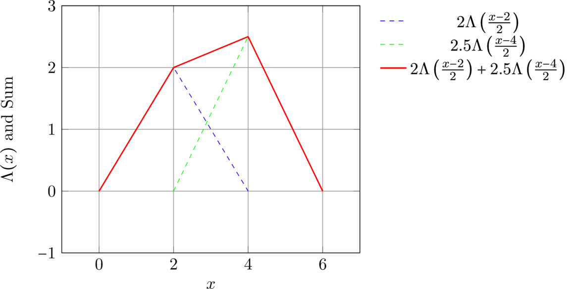
The signal is a sum of two scaled and shifted $\Lambda$ functions:

![\[2\Lambda\left(\frac{x – 2}{2}\right) + 2.5\Lambda\left(\frac{x – 4}{2}\right)\]](images/quicklatex.com-b0f6260f1b6510207251aa53f96b2c73_l3.png)

Equivalently,

Exploring $\Lambda(x)$

Before solving the main problem, let us review the Fourier transform of the scaled triangular function $\Lambda\left(\frac{x}{c}\right)$.

Using the Fourier transform convention

the transform of the scaled triangular function is

![\[\mathcal{F}\left(\Lambda\left(\frac{x}{c}\right)\right) = \int_{-c}^{c} \Lambda\left(\frac{x}{c}\right) e^{-i 2 \pi s x} dx \quad \text{(1)}\]](images/quicklatex.com-05b79106320954fb7eef89c3f87aaaf5_l3.png)

With the substitution $y = \frac{x}{c}$, so that $x = cy$ and $dx = c\,dy$, this becomes

Since $\mathcal{F}\{\Lambda(x)\}(s) = \mathbf{sinc}^2(s)$ under this convention, we obtain

![\[\mathcal{F}\left(\Lambda(y)\right) = c \mathbf{sinc}^2(cs) \quad \text{(2)}\]](images/quicklatex.com-ecb2d36ab9f5f25c720e90f49837e3e8_l3.png)

More precisely,

where $\mathbf{sinc}(s)=\frac{\sin(\pi s)}{\pi s}$.

Generalizing the Fourier Transform

Next, we use the shift property of the Fourier transform:

![\[g(t-b) \xleftrightarrow{} e^{-j 2 \pi b s} G(s)\]](images/quicklatex.com-0678d84a6b349d115d898146cb781849_l3.png)

Therefore, for a scaled and shifted triangular function,

![\[\mathcal{F}\left(a\Lambda\left(\frac{x-b}{c}\right)\right) = a c \, e^{-j 2 \pi b s} \mathbf{sinc}^2(cs) \quad \text{(3)}\]](images/quicklatex.com-f5d841f9702b9b603e9c647345c29bac_l3.png)

or, in inline form,

Solving the Problem

For the first term,

so

For the second term,

so

By linearity, the Fourier transform of the full signal is

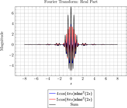
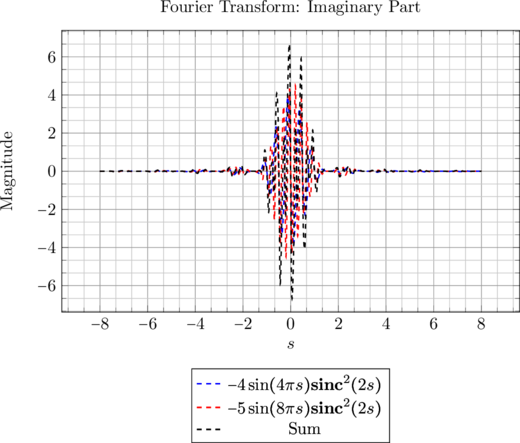
![\[\mathcal{F}\left(2\Lambda\left(\frac{x-2}{2}\right) + 2.5\Lambda\left(\frac{x-4}{2}\right)\right) = 4 e^{-j 4 \pi s} \mathbf{sinc}^2(2s) + 5 e^{-j 8 \pi s} \mathbf{sinc}^2(2s) \quad \text{(4)}\]](images/quicklatex.com-546cfaf2c99a9b6a1325fce56d5f98b1_l3.png)

That is,

This can also be factored as

Below are visual representations of the Fourier transform of this signal, showing its real and imaginary components:

Conclusion

We have solved the Fourier transform of a signal built from shifted and scaled triangular functions. The key tools were the known transform pair for $\Lambda(x)$, the scaling property, the shift property, and linearity. Together, these rules reduce what first appears to be a complicated signal into a direct combination of phase-shifted $\mathbf{sinc}^2$ terms.

As this series continues, we will explore more examples and applications of the Fourier transform. Until then, keep transforming.