Physics, Pattern, Prediction and Python

Table of Contents

Introduction

Physics is a discipline of patterns: repeated observations are turned into compact laws, and those laws are tested by prediction. Python is useful in this workflow because it lets us move between symbolic reasoning, numerical simulation, visualization, and machine learning without changing tools too often.

This note sketches a practical map from physical ideas to computational methods. It is not a replacement for a textbook, but it gives a structure for studying physics with code: identify the model, write down the mathematical objects, choose an approximation when exact calculation is impossible, and check the result against units, limiting cases, and known examples.

Pattern recognition and machine learning

Pattern recognition begins with data. In physics, the data may be a time series from an oscillator, a spectrum from an experiment, a set of particle tracks, or simulated samples from a model. The basic workflow is stable:

Define the observable and its units.
Clean the data without destroying the signal.
Choose a model class.
Fit parameters on training data.
Validate on held-out data or known physical limits.
Inspect residuals and uncertainty.

Machine learning can help when the mapping from input to output is hard to write explicitly. For example, a neural network can classify phases of matter from configurations, approximate a potential-energy surface, or learn a surrogate model for an expensive simulation. The important caution is that a successful predictor is not automatically a physical explanation. A physics model should also respect constraints such as conservation laws, symmetries, dimensional consistency, and causality.

A minimal reproducible check in Python is to separate the physical model from the fitting code:

import numpy as np
from sklearn.linear_model import LinearRegression

# Example: y = a x + b with noisy observations.
rng = np.random.default_rng(42)
x = np.linspace(0, 10, 100)
y = 2.5 * x - 1.0 + rng.normal(scale=0.8, size=x.shape)

model = LinearRegression()
model.fit(x.reshape(-1, 1), y)

print(model.coef_[0], model.intercept_)

Before trusting the result, check whether the fitted parameters have the expected dimensions and whether the residuals show structure. If the residuals are patterned, the model is missing physics.

Classical physics

Classical physics is the natural starting point because many systems can be described by positions, velocities, forces, fields, and energy. Newtonian mechanics gives the familiar equation

F = m a

For a system with position x(t), the computational problem often becomes solving an ordinary differential equation. For a damped oscillator,

m x'' + c x' + k x = 0

we can integrate the system numerically by rewriting it as first-order equations:

import numpy as np
from scipy.integrate import solve_ivp

m = 1.0
c = 0.2
k = 4.0

def oscillator(t, state):
    x, v = state
    dxdt = v
    dvdt = -(c / m) * v - (k / m) * x
    return [dxdt, dvdt]

solution = solve_ivp(
    oscillator,
    t_span=(0.0, 20.0),
    y0=[1.0, 0.0],
    max_step=0.05,
)

print(solution.t.shape, solution.y.shape)

The same pattern appears in electromagnetism, fluid dynamics, and continuum mechanics: write down governing equations, choose boundary and initial conditions, select a numerical method, and verify conservation or stability where possible.

Useful checks include:

In the limit c = 0, the oscillator should conserve energy.
Smaller time steps should not radically change the result.
Parameters should carry consistent units.
Numerical artifacts should not be mistaken for physical effects.

Quantum mechanics and quantum computing

Quantum mechanics replaces deterministic trajectories with states, operators, amplitudes, and measurement probabilities. A pure state is represented by a vector |psi>, and observables are represented by operators. The Schrodinger equation describes time evolution:

i hbar d|psi>/dt = H |psi>

For finite-dimensional systems, the Hamiltonian H can be represented as a matrix. A two-level system is the simplest useful example:

import numpy as np
from scipy.linalg import expm

hbar = 1.0
sigma_x = np.array([[0, 1], [1, 0]], dtype=complex)

H = 0.5 * sigma_x
psi0 = np.array([1, 0], dtype=complex)

def evolve(t):
    U = expm(-1j * H * t / hbar)
    return U @ psi0

psi_t = evolve(np.pi)
probabilities = np.abs(psi_t) ** 2
print(probabilities)

Quantum computing uses controlled quantum evolution as a computational resource. A qubit is a two-level quantum system, and gates are unitary operations. The practical questions are usually:

How is the state prepared?
Which unitary operations are applied?
What measurement is performed?
How many samples are needed to estimate the result?
What noise model is relevant?

When using a quantum computing library, verify the installed version locally and read the current documentation, because APIs and supported devices change over time.

Relativity and tensor

Relativity is built around objects that transform consistently between coordinate systems. Tensors provide the language for this. In general relativity, spacetime curvature is related to energy and momentum through the Einstein field equation:

(1) Einstein field equation

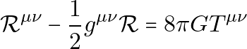
Here g is the metric tensor, R is curvature, T is the stress-energy tensor, and G is Newton’s gravitational constant. The equation is compact, but solving it usually requires symmetry assumptions, approximations, or numerical relativity.

Tensor notation keeps track of how components transform. For example:

(2) Mixed tensor notation

A practical computational habit is to separate the abstract object from its coordinate representation. For example, when working with a metric tensor, check:

The coordinate chart being used.
The metric signature convention.
Whether indices are covariant or contravariant.
Whether constants such as c are set to 1.
Whether units are geometrized or SI.

Tensor packages can automate index manipulation, but they do not remove the need to understand conventions.

Cosmology and astrophysics

Cosmology applies general relativity, thermodynamics, nuclear physics, and statistical inference to the universe as a whole. The standard large-scale model assumes homogeneity and isotropy, which leads to the Friedmann-Lemaitre-Robertson-Walker metric and the Friedmann equations.

Astrophysics works across a wide range of scales: stellar structure, compact objects, galaxies, gravitational waves, and cosmic background radiation. Python is commonly used for units, coordinate transforms, catalog handling, fitting, and visualization.

A durable computational habit is to make units explicit. With astropy, for example:

from astropy import units as u
from astropy.constants import G, M_sun

mass = 1.0 * M_sun
radius = 6.96e8 * u.m
escape_velocity = (2 * G * mass / radius) ** 0.5

print(escape_velocity.to(u.km / u.s))

This style prevents many silent errors. A number may look plausible while its units are wrong.

Statistical mechanics

Statistical mechanics connects microscopic states with macroscopic quantities such as temperature, entropy, pressure, and free energy. The central object is often the partition function:

Z = sum_i exp(-beta E_i)

where beta = 1 / (k_B T). Once Z is known, thermodynamic quantities can be derived from it. For small systems, the sum can be computed directly:

import numpy as np

k_B = 1.0
T = 2.0
beta = 1.0 / (k_B * T)
energies = np.array([0.0, 1.0, 2.0, 4.0])

weights = np.exp(-beta * energies)
Z = weights.sum()
probabilities = weights / Z
mean_energy = np.sum(probabilities * energies)

print(Z, probabilities, mean_energy)

For large systems, direct enumeration becomes impossible. Monte Carlo methods, molecular dynamics, and approximation techniques are then used. As always, the numerical result should be checked against limiting cases: high temperature, low temperature, small system size, or analytically solvable models.

Implementation with Python

Python is useful because the ecosystem covers several layers of physics work:

NumPy for arrays and linear algebra.
SciPy for integration, optimization, sparse matrices, and special functions.
Matplotlib for plotting.
SymPy for symbolic mathematics.
scikit-learn for standard machine learning workflows.
Domain libraries for quantum mechanics, relativity, astrophysics, and thermodynamics.

A reliable environment starts with an isolated virtual environment and explicit dependencies:

python -m venv .venv
source .venv/bin/activate
python -m pip install --upgrade pip
python -m pip install numpy scipy matplotlib sympy scikit-learn

Then verify versions locally:

python - <<'PY'
import numpy, scipy, sympy
print('numpy', numpy.__version__)
print('scipy', scipy.__version__)
print('sympy', sympy.__version__)
PY

PennyLane

PennyLane is a Python library for differentiable quantum programming. It is useful for experiments that combine quantum circuits with optimization or machine learning. A typical workflow is:

Choose a device or simulator.
Define a quantum node.
Build a parameterized circuit.
Evaluate an expectation value.
Optimize parameters with a classical optimizer.

Always check the installed version and supported devices locally, because quantum software changes quickly.

SymPy

SymPy is useful when the mathematical expression matters as much as the numerical result. It can simplify expressions, differentiate symbolically, solve equations, and generate numerical functions.

import sympy as sp

x, k, m = sp.symbols('x k m', positive=True)
V = sp.Rational(1, 2) * k * x**2
force = -sp.diff(V, x)

print(force)

Symbolic work is especially helpful for deriving equations before committing to a numerical implementation.

QuTiP, einsteinpy, astropy, thermopy

QuTiP is used for quantum dynamics and open quantum systems. It is useful when density matrices, master equations, and quantum operators are central.

einsteinpy focuses on relativity calculations such as geodesics, metrics, and symbolic tensor operations.

astropy is a mature library for astronomy and astrophysics, especially units, coordinates, constants, time, and data formats.

thermopy is used for thermodynamic calculations. Before relying on it in a project, verify its current maintenance status and compatibility with your Python version.

For any domain package, the practical rule is the same: install it in an isolated environment, run a minimal example from the current documentation, and write a small verification test that checks a known result.