
We will use this simple data set  throughout the tutorial. If we use the fourth column as the label, the third column is the feature; if we use the third column as the label, the fourth column is the feature.
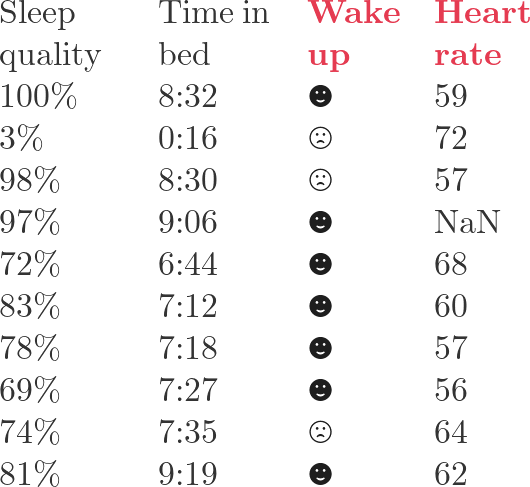
Table of Contents
Boosting
Boosting is an additive modeling strategy. Instead of training one complex model at once, we train many simple models sequentially. Each new model tries to correct what the current ensemble still gets wrong.
Write the prediction after step m as
where F_{m-1} is the current model, f_m is the new weak learner, and \eta is the learning rate. In tree boosting, f_m is usually a regression tree. The important idea is that the tree does not learn the original target directly; it learns the direction in which the current prediction should move.
For squared-error regression this direction is easy to see:
so the negative gradient is
That is just the residual. This is why gradient boosting can be introduced as “fit the next tree to the residuals.” For other losses, the same idea still works, but the residual becomes a gradient-derived pseudo-residual.
Gradient Boost for Regression
The loss function of gradient boosting can be written as
Here \hat{y}_i^{(t-1)} is the prediction before adding the new tree, f_t(x_i) is the update from the new tree, and \Omega(f_t) is a regularization term. To build intuition, ignore regularization first:
For squared error,
The derivative with respect to the current prediction is
Therefore the negative gradient is
which is exactly the residual. A regression boosting iteration is therefore:
- Predict with the current ensemble.
- Compute residuals or negative gradients.
- Fit a new tree to those residuals.
- Add the tree to the ensemble, usually multiplied by a learning rate.
This explains the bridge from ordinary residual fitting to gradient boosting: residuals are a special case of negative gradients.
Gradient Boost for Classification
Caveat: to avoid heavy notation, the summation symbol \sum is sometimes omitted below. The derivation is for binary classification.
For a binary classification problem, define odds as
The probability is
With simple algebra,
This is the logistic sigmoid applied to the log-odds. Let
Then
Use binary cross entropy as the loss:
We want to find \gamma that minimizes the loss:
We could work directly on the loss and solve
but that becomes cumbersome. A second-order Taylor approximation gives a cleaner update. Around the current score F_{m-1},
where
Set the derivative with respect to \gamma to zero:
This gives
so the optimal local update is
For binary cross entropy, the first derivative with respect to F = \log(\text{odds}) is
With some illustration:

The second derivative of \mathcal{L} with respect to \log(\text{odds}) is
Therefore, for one observation,
For a leaf containing many observations, the Newton-style update aggregates gradients and Hessians:
This is the practical bridge from gradient boosting classification to XGBoost.
XGBoost
XGBoost keeps the additive tree model but makes the objective more explicit and regularized. At boosting round t, it minimizes
where the tree regularization is commonly written as
Here T is the number of leaves, w_j is the score of leaf j, \gamma penalizes adding leaves, and \lambda is L2 regularization on leaf weights.
Using the second-order Taylor approximation,
where
For a fixed tree structure, each sample falls into one leaf. Let I_j be the set of samples in leaf j, and define
The objective for leaf j becomes
The best leaf weight is therefore
This is the XGBoost version of the -g/h update. The regularization term \lambda prevents very large leaf scores when the Hessian is small.
The corresponding score of a tree structure is
When splitting a leaf into left and right children, XGBoost evaluates the gain:
A split is useful when this gain is positive and large enough to justify the extra complexity. This is why XGBoost is not just “gradient boosting with trees”; it is gradient boosting with second-order information, explicit leaf scoring, and regularized split selection.
A minimal way to inspect these ideas in Python is:
import numpy as np

# Binary labels and current probabilities from the current ensemble.
y = np.array([1, 0, 0, 1, 1], dtype=float)
p = np.array([0.55, 0.40, 0.48, 0.70, 0.62], dtype=float)

# Logistic-loss gradient and Hessian with respect to the log-odds score F.
g = p - y
h = p * (1 - p)

lambda_l2 = 1.0
leaf_weight = -g.sum() / (h.sum() + lambda_l2)

print(g)
print(h)
print(leaf_weight)
The exact numbers depend on the current predictions and on which samples fall into the leaf. The formula is stable: compute gradients, compute Hessians, aggregate them by leaf, then use -G / (H + lambda).
Reference
- Dana D. Sleep Data Personal Sleep Data from Sleep Cycle iOS App. Kaggle. https://www.kaggle.com/danagerous/sleep-data#