
This note is a worked introduction to the Quantum Approximate Optimization Algorithm (QAOA), with the algebraic steps written out rather than left as exercises. The focus is the standard Ising-style formulation used for combinatorial optimization, how it connects to adiabatic quantum computation, how the circuit is built, and how to evaluate the operator identities that appear in the simplest derivations.
Table of Contents
The Problem Definition
QAOA is a variational quantum algorithm for approximately solving optimization problems. A classical objective function is encoded into a cost Hamiltonian \(C\), and the algorithm prepares a parameterized quantum state whose measurement distribution favors low-cost or high-cost bit strings, depending on the sign convention.
For a binary optimization problem, write a candidate solution as a bit string
The objective function assigns a real value \(C(z)\) to each bit string. In QAOA we promote this classical function to a diagonal quantum operator
The algorithm also uses a mixing Hamiltonian, usually
where \(X_j\) is the Pauli \(X\) operator acting on qubit \(j\). For depth \(p\), the QAOA state is
where
is the uniform superposition over all computational basis states. The classical outer loop chooses the angles
to optimize the expectation value
For a maximization problem, one tries to maximize \(F_p\). For a minimization problem, either minimize the same expression or change the sign of the cost Hamiltonian.
Transverse Field Ising Model
Many QAOA examples use an Ising Hamiltonian because binary variables can be represented naturally by Pauli \(Z\) operators. For two qubits, a common interaction term is
A graph-based cost Hamiltonian often has the form
possibly plus one-local fields
The transverse-field part is the mixer
So the two alternating pieces in QAOA are:
- a diagonal Ising cost evolution \(e^{-i\gamma C}\), and
- a transverse-field mixing evolution \(e^{-i\beta B}\).
The useful point is that many terms commute. All \(Z_iZ_j\) terms are diagonal, so they commute with one another. All \(X_i\) terms also commute with one another because they act on different qubits. This lets us implement the exponentials as products of one-qubit and two-qubit gates.
Adiabatic Quantum Computation
QAOA can be viewed as a digitized, variational version of adiabatic quantum computation.
In the adiabatic picture, we begin with an easy Hamiltonian whose ground state is easy to prepare, for example
Its ground state is \(|+\rangle^{\otimes n}\). We then slowly change the Hamiltonian toward the problem Hamiltonian \(H_C\):
where \(s(0)=0\) and \(s(T)=1\). If the interpolation is slow enough and the spectral gap behaves well, the adiabatic theorem says the state approximately follows the instantaneous ground state.
QAOA replaces this continuous process with alternating pulses:
At large depth \(p\), the sequence resembles a Trotterized adiabatic path. At small depth, the angles are treated as free variational parameters and optimized directly.
Circuit Design
For one QAOA layer, the circuit has three parts.
- Prepare the initial state:
- Apply the cost unitary:
For an Ising edge \((i,j)\), the two-qubit term is
A standard decomposition is:
CNOT(i, j)
RZ(2 gamma w_ij) on j
CNOT(i, j)
The sign of the angle depends on the convention used by the quantum SDK for \(R_Z(\theta)\). Always verify it from the local definition of the gate.
- Apply the mixer unitary:
Since many SDKs define
this is usually implemented as
RX(2 beta) on every qubitAgain, verify the sign and factor of two against the local SDK definition.
The full depth-\(p\) circuit repeats the cost and mixer blocks:
H on every qubit
for layer = 1..p:
    apply cost unitary with gamma[layer]
    apply mixer unitary with beta[layer]
measure
Coding
A minimal implementation has three moving parts:
- a function that builds the QAOA circuit for given parameters,
- a function that estimates the expected cost from measurement counts, and
- a classical optimizer that updates the angles.
Pseudocode:
def qaoa_circuit(graph, gammas, betas):
    circuit = QuantumCircuit(len(graph.nodes))

    for q in graph.nodes:
        circuit.h(q)

    for gamma, beta in zip(gammas, betas):
        for i, j, weight in graph.edges(data="weight", default=1.0):
            circuit.cx(i, j)
            circuit.rz(2 * gamma * weight, j)
            circuit.cx(i, j)

        for q in graph.nodes:
            circuit.rx(2 * beta, q)

    circuit.measure_all()
    return circuit
To evaluate a bit string, define the same cost function used to build the Hamiltonian. For example, for an Ising objective:
def spin(bit):
    return 1 if bit == "0" else -1


def ising_cost(bitstring, edges):
    total = 0.0
    for i, j, weight in edges:
        total += weight * spin(bitstring[i]) * spin(bitstring[j])
    return total
Then estimate the expectation value from counts:
def expected_cost(counts, edges):
    shots = sum(counts.values())
    return sum(ising_cost(bits, edges) * count / shots for bits, count in counts.items())
This is deliberately SDK-neutral. In a real implementation, check the bit-ordering convention of the backend or simulator. Some frameworks return bit strings with the visual order reversed relative to qubit indices.
Trivial State Preparation
After several days of thinking and researching, I decided to answer my own question.
N.B. The tensor product symbol  is omitted when there is no risk of confusion, especially when the index is different. In symbols,
 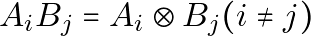 .
.
First, for the case 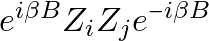 , consider only qubit
  , where
 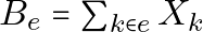 . Since
  and
and  act on different qubits,

Now,
Thus,
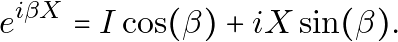
Hence,
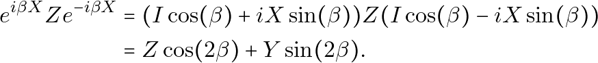
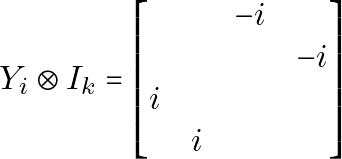
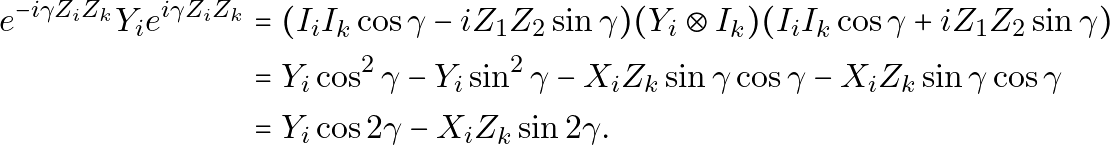
For the transverse-field Ising Hamiltonian, consider 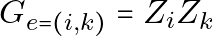 .
.
For  , it can be evaluated as
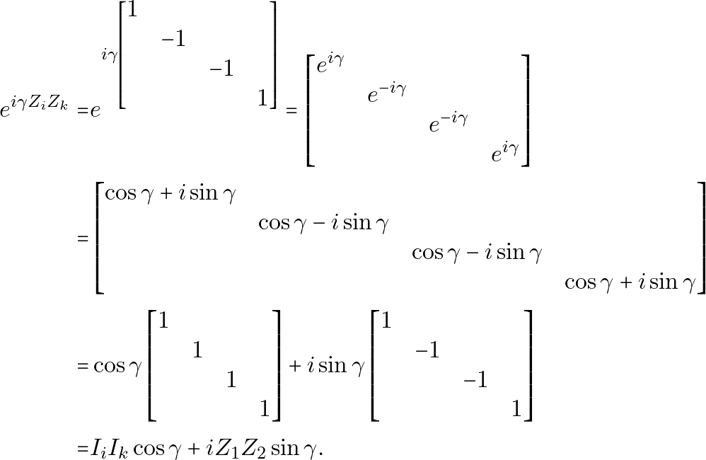
We can calculate two-qubit operations independently:

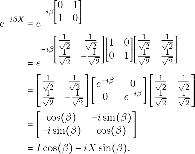
Numerically, if you cannot convince yourself,
and
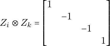
and
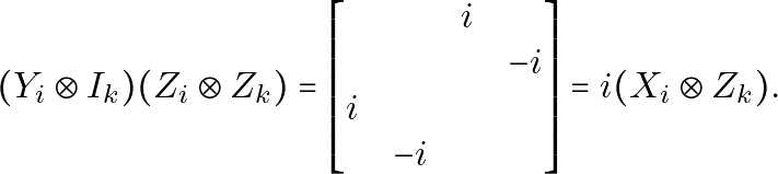
Now, for a more specific example,
Q.E.D.
Reference
- Choi J, Kim J. A Tutorial on Quantum Approximate Optimization Algorithm (QAOA): Fundamentals and Applications. In: 2019 International Conference on Information and Communication Technology Convergence (ICTC). IEEE; 2019. doi:10.1109/ictc46691.2019.8939749