The Unfolding Universe of Quantum Field Theory: A Journey Through Exercise 1.3 Part 1

The world of Quantum Field Theory (QFT) is nothing short of mesmerizing: a cosmic dance of mathematics and physics that unearths the deepest workings of the universe. Right now, I am entranced by the book Quantum Field Theory for the Gifted Amateur, an intellectual odyssey that has opened new horizons for me.

I’d like to share an intimate part of this journey: an exploration of Exercise 1.3. This exercise delves into the intricacies of functionals and their derivatives, a mathematical arena where classical calculus meets the subtle beauty of functional analysis.

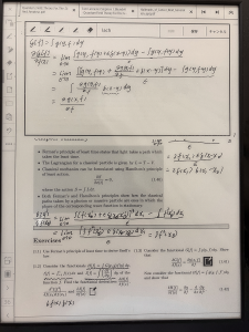
Table of Contents

The Exercise

Consider the functional

\[G[f] = \int g(y, f)\,\mathrm{d}y.\]

Show that

\[\frac{\delta G[f]}{\delta f(x)} = \frac{\partial g(x, f)}{\partial f}.\]

We are also asked to extend this idea to more complex functionals involving $f’$ and $f”$, the first and second derivatives of $f$ with respect to $y$.

Step 1: Setting Up the Functional

The first functional can be written more explicitly as

\[G[f] = \int g(y, f(y))\,\mathrm{d}y.\]

To find the functional derivative $\delta G[f]/\delta f(x)$, we perturb the function $f$ at the point $x$. One convenient way to express that perturbation is with the Dirac delta function:

\[f(y) \rightarrow f(y) + \epsilon\delta(x-y),\]

where $\epsilon$ is a small number. The functional derivative is then defined by

\[\frac{\delta G[f]}{\delta f(x)} = \lim_{\epsilon \to 0} \frac{G[f(y)+\epsilon\delta(x-y)] – G[f(y)]}{\epsilon}.\]

Step 2: Delving Into the Derivative

Substituting the functional into the definition gives

\[\begin{aligned} \frac{\delta G[f]}{\delta f(x)} &= \lim_{\epsilon \to 0} \frac{\int g(y, f(y)+\epsilon\delta(x-y))\,\mathrm{d}y – \int g(y, f(y))\,\mathrm{d}y}{\epsilon}. \end{aligned}\]

Expanding $g$ to first order in $\epsilon$,

\[g(y, f(y)+\epsilon\delta(x-y)) = g(y, f(y)) + \epsilon\frac{\partial g(y, f)}{\partial f}\delta(x-y) + O(\epsilon^2).\]

Therefore,

\[\begin{aligned} \frac{\delta G[f]}{\delta f(x)} &= \lim_{\epsilon \to 0} \frac{\int \left[g(y, f(y)) + \epsilon\frac{\partial g(y, f)}{\partial f}\delta(x-y)\right]\,\mathrm{d}y – \int g(y, f(y))\,\mathrm{d}y}{\epsilon} \\ &= \int \frac{\partial g(y, f)}{\partial f}\delta(x-y)\,\mathrm{d}y \\ &= \frac{\partial g(x, f)}{\partial f}. \end{aligned}\]

So we find exactly what the exercise asks us to show:

\[\frac{\delta G[f]}{\delta f(x)} = \frac{\partial g(x, f)}{\partial f}.\]

Extending the Result to $f’$

Now suppose the functional depends on the derivative of the function:

\[G[f] = \int g(y, f, f’)\,\mathrm{d}y.\]

A small variation $f \rightarrow f + \epsilon\eta$ gives

\[\delta G = \epsilon\int\left( \frac{\partial g}{\partial f}\eta + \frac{\partial g}{\partial f’}\eta’ \right)\mathrm{d}y.\]

The term involving $\eta’$ is not yet in the form needed for a functional derivative, so we integrate by parts:

\[\int \frac{\partial g}{\partial f’}\eta’\,\mathrm{d}y = \left[\frac{\partial g}{\partial f’}\eta\right]_{\text{boundary}} – \int \frac{\mathrm{d}}{\mathrm{d}y}\left(\frac{\partial g}{\partial f’}\right)\eta\,\mathrm{d}y.\]

If the variation vanishes at the boundary, the boundary term is zero. Then

\[\delta G = \epsilon\int\left[ \frac{\partial g}{\partial f} – \frac{\mathrm{d}}{\mathrm{d}y}\left(\frac{\partial g}{\partial f’}\right) \right]\eta\,\mathrm{d}y.\]

Thus,

\[\frac{\delta G[f]}{\delta f(x)} = \frac{\partial g}{\partial f} – \frac{\mathrm{d}}{\mathrm{d}x}\left(\frac{\partial g}{\partial f’}\right),\]

with all quantities evaluated at $y=x$.

Extending the Result to $f”$

For a functional depending on the second derivative,

\[G[f] = \int g(y, f, f’, f”)\,\mathrm{d}y,\]

the variation is

\[\delta G = \epsilon\int\left( \frac{\partial g}{\partial f}\eta + \frac{\partial g}{\partial f’}\eta’ + \frac{\partial g}{\partial f”}\eta” \right)\mathrm{d}y.\]

The $\eta’$ term is handled by one integration by parts. The $\eta”$ term requires two integrations by parts:

\[\int \frac{\partial g}{\partial f”}\eta”\,\mathrm{d}y = \left[\frac{\partial g}{\partial f”}\eta’ – \frac{\mathrm{d}}{\mathrm{d}y}\left(\frac{\partial g}{\partial f”}\right)\eta\right]_{\text{boundary}} + \int \frac{\mathrm{d}^2}{\mathrm{d}y^2}\left(\frac{\partial g}{\partial f”}\right)\eta\,\mathrm{d}y.\]

Assuming the boundary terms vanish, we obtain

\[\frac{\delta G[f]}{\delta f(x)} = \frac{\partial g}{\partial f} – \frac{\mathrm{d}}{\mathrm{d}x}\left(\frac{\partial g}{\partial f’}\right) + \frac{\mathrm{d}^2}{\mathrm{d}x^2}\left(\frac{\partial g}{\partial f”}\right).\]

This is the Euler-Lagrange pattern that appears throughout classical field theory and quantum field theory: each derivative of the field contributes a term with alternating signs after integration by parts.

Reflection

This exercise is a profound exploration of how functionals interact with their derivatives, providing a mathematical vocabulary for discussing the subtleties of Quantum Field Theory. It is akin to learning the syntax of an intricate language, each symbol a poetic word in a story that is constantly unfolding.

My journey through the universe of Quantum Field Theory continues, and this exercise is a small but essential step: it shows how local variations of a function turn an integral expression into a pointwise equation, the basic move behind the equations of motion in field theory.